The Linguistic Covariance Space of Undergraduate STEM Programs at Virginia Commonwealth University

Mapping textual input into quantitative spaces facilitates statistical analyses supporting decision analytics. Here, university course descriptions are mapped onto numerical spaces and used to define the landscape of academic covariance based upon CORE class components.

As part of my book project, Intentional Curriculum Design: Data-Centric Approaches for STEM Curricula, I am analyzing the current landscape of university curricula based on the descriptions of all CORE classes—those offerings in each degree program that all students must take. This is the third installment of posts describing how we can characterize the linguistic taxonomy of STEM programs. The first two posts describe data acquisition and mapping textual components onto quantitative spaces.

1. Linguistic Taxonomies of STEM Programs: Parsing Course Descriptions
2. Frequency-Dependent Linguistic Embedding of Course Descriptions

Here, I describe the basics of how to configure these data and perform an analysis that describes the Conditional Covariance of these programs—a technique I developed for population analyses based upon genetic covariance and evolutionary histories (see here, here, here, here, here, and here for the underlying theory and a variety of examples).

Conditional Covariance

Conditional covariance is a statistical concept that describes the extent to which two variables change together, given the presence of a third variable. This approach has been extended to produce a minimal covariance topology, or network, that describes the underlying system. In population genetics, this topology displays the evolutionary history of the set of populations. In the context of undergraduate STEM programs, this topology describes the differences and taxonomies of all STEM programs based on the specific course components that all students must take. This linguistic approach has been used to examine the relative position of emergent scientific disciplines such as Landscape Genetics (see Dyer 2015).The data created in the previous post can be used to construct the linguistic covariance matrix, which reflects the relationships between programs based on the interconnectedness of shared courses—or alternative courses with similar linguistic structures. Only CORE classes are used in this construction as they are the foundation by which the State Council of Higher Education of Virginia (SCHEV) defines these academic programs. This is beneficial for comparative purposes across programs at VCU and comparisons across programs at different institutions across the Commonwealth of Virginia.

The goal is to develop tools that enhance our understanding of a curriculum's design and provide a foundation for data-driven development. By identifying areas of strong connectivity or potential gaps, educators and administrators can make informed decisions to optimize students' learning pathway curriculum decisions, ensuring that the curriculum remains cohesive and aligned with educational goals. Moreover, once the topological space of CORE programs is specified, students may use this configuration to select in-program and open electives to maximize their degree progression in specific academic directions. For example, an Environmental Studies student may be interested in quantitative policy analysis and desire to choose electives that will bring the totality of their degree progression from the CORE of Environmental Studies towards Urban Studies, Political Science, Economics, and Management. What does that specific mix of disciplines look like, and how should they choose courses that cover the linguistic landscape encompassed by those domain-specific pursuits? This approach will help, as will the application that I will describe in a later installment.

Defining Academic Programs

In the previous post, I mapped all courses at VCU onto a quantitative space. I went into the VCU Bulletin and looked at all the STEM fields we have (I made some distinctions about what is and what is not STEM, based upon Googling if the National Science Foundation considers something STEM-related). There is no official list by CIP-Code, so I'm sure I made some mistakes here. Please do not flame me if I misallocated your preferred profession. In the end, my goal in this series is to provide a demonstration of how this can be done. The publication of this work will have all programs (STEM and non-STEM), and we will see if the resulting topology supports this distinction.I made the following assumptions when selecting data for this model.

1. All classes that are CORE (e.g., every student must take) were included in each program.
2. I disregarded the General Education curriculum, as it is a "select X credits from the following list" approach. This means individuals in the same major may have different general education requirements. Given that the General Education requirements total 30 credits, it may be a significant component for some majors and would primarily add error variance to the overall model.
3. If there are a pair of options, this is not uncommon. For example, in Environmental Studies, one can take PHYS 201: General Physics I or PHYS 207: University Physics I. I always selected the first option, which is most commonly the one with a smaller number.
4. If programs have a "Select X credits from the following list" option, I included none because they are not CORE (e.g., guaranteed that every graduate will have that class). There is an argument to be made that we should include all classes but assign an a priori weight to them. In my other work, I find that this cleans up some dirty data sets but does not qualitatively impact the interpretation of the output; perhaps subsequent exploration of this approach is necessary.

So, I encoded these programs based on the classes and loaded them into my environment.

workspace.load("data/vcu_courses.rda")
source("data/vcu_programs.R")

At VCU, we have 44 undergraduate programs that could be considered STEM (I may have missed a few). Some majors have several options, not quite tracks, but different majors under the same rubric. For example, Bioinformatics (BNFO) has separate Computational(bnfo_comp), Genomic (bnfo_genomic), and Statistical (bnfo_stat) programs with different (though mostly overlapping) sets of classes. In these cases, I added all three programs.

 names(programs)

 [1] "anthro"         "biol"           "biomedEng"      "bnfo_comp"     
 [5] "bnfo_genomic"   "bnfo_stat"      "chemLSEng_chem" "chemLSEng_lfsc"
 [9] "chem_biochem"   "chem_chemsci"   "chem_modeling"  "chem_profchem" 
[13] "compEng"        "compSci"        "compSci_cyber"  "compSci_data"  
[17] "compSci_eng"    "elecEng"        "envs"           "frsc_bio"      
[21] "frsc_chem"      "frsc_phys"      "hpex_exercise"  "hpex_health"   
[25] "math_applied"   "math_bio"       "math_gen1"      "math_gen2"     
[29] "math_math"      "math_teacher"   "mechEng"        "mechEng_nuc"   
[33] "phys"           "phys_nano"      "phys_premed"    "psyc"          
[37] "psyc_addic"     "psyc_applied"   "psyc_grad"      "psyc_lfsc"     
[41] "psyc_urban"     "socy"           "ssor_or"        "ssor_stat" 

Here is what the core classes for ENVS majors look like:

  programs$envs

 [1] "BIOL 151" "BIOL 152" "BIOL 317" "BIOZ 151" "BIOZ 152" "CHEM 101"
 [7] "CHEM 102" "CHEZ 101" "CHEZ 102" "ECON 325" "ENVS 101" "ENVS 102"
[13] "ENVS 105" "ENVS 222" "ENVS 311" "ENVS 321" "ENVS 330" "ENVS 343"
[19] "ENVS 355" "ENVS 401" "ENVS 499" "MATH 151" "PHYS 201"

VCU lists 2863 potential courses, though I suspect many of these are not taught (or at least recently been offered). Looking at CORE credit load by program, we see a wide range of requirements.

data.frame( Program = names(programs), 
            CourseCount = NA,
            Credits = NA) -> df 

for( program in df$Program ) { 
  core <- programs[[program]]
  classes <- vcu_courses[ vcu_courses$class %in% core, ]
  credits <- sum(as.numeric(classes$hours) )
  df$CourseCount[ df$Program == program ] <- length( core )
  df$Credits[ df$Program == program ] <- credits 
}

df |> 
  ggplot( aes(Program, Credits) ) + 
  geom_col() +
  scale_x_discrete(guide = guide_axis(angle = 45)) +
  geom_hline( yintercept = mean( df$Credits ), col="red", lty=2) + 
  xlab("Academic Program") + ylab("CORE Credits") +
  theme_minimal()

Linguistic Mapping

Next, I define the linguistic spaces for each major by weighing the linguistic vector for each course by the number of credits in the class, creating a matrix of linguistic weights for each major. In the case of ENVS, there are 23 core classes, and the linguistic weights from the previous post showed 551 columns of data for each class. 

For context, the data mapping we are using has the following characteristics that are essential to understand when we start interpreting the outcomes:

Dimensionality

Each program, for example, the BS in ENVS, statistically defines a point cloud in a high-dimensional linguistic space. This specific program has 23 points defined in 551 orthogonal axes. The number of points in this space depends on the CORE classes. The Psychology program requires nine courses (with room for "choose from the following" and many electives), whereas the Mechanical and Nuclear Engineering program requires 42 courses (e.g., there are no electives).

Location

Different classes may have a very close location in this linguistic space. The first ENVS course has the following description.

ENVS 101. INTRODUCTION TO ENVIRONMENTAL STUDIES I. 3 HOURS.  Semester course; 3 lecture hours. 3 credits. Enrollment is restricted to environmental studies majors. Study of contemporary issues related to environmental studies, including sustainability, biological conservation, global change, and an overview of the core earth systems

If we look at the Euclidean distance between ENVS 101 and all the rest, we see the following distribution of distances:

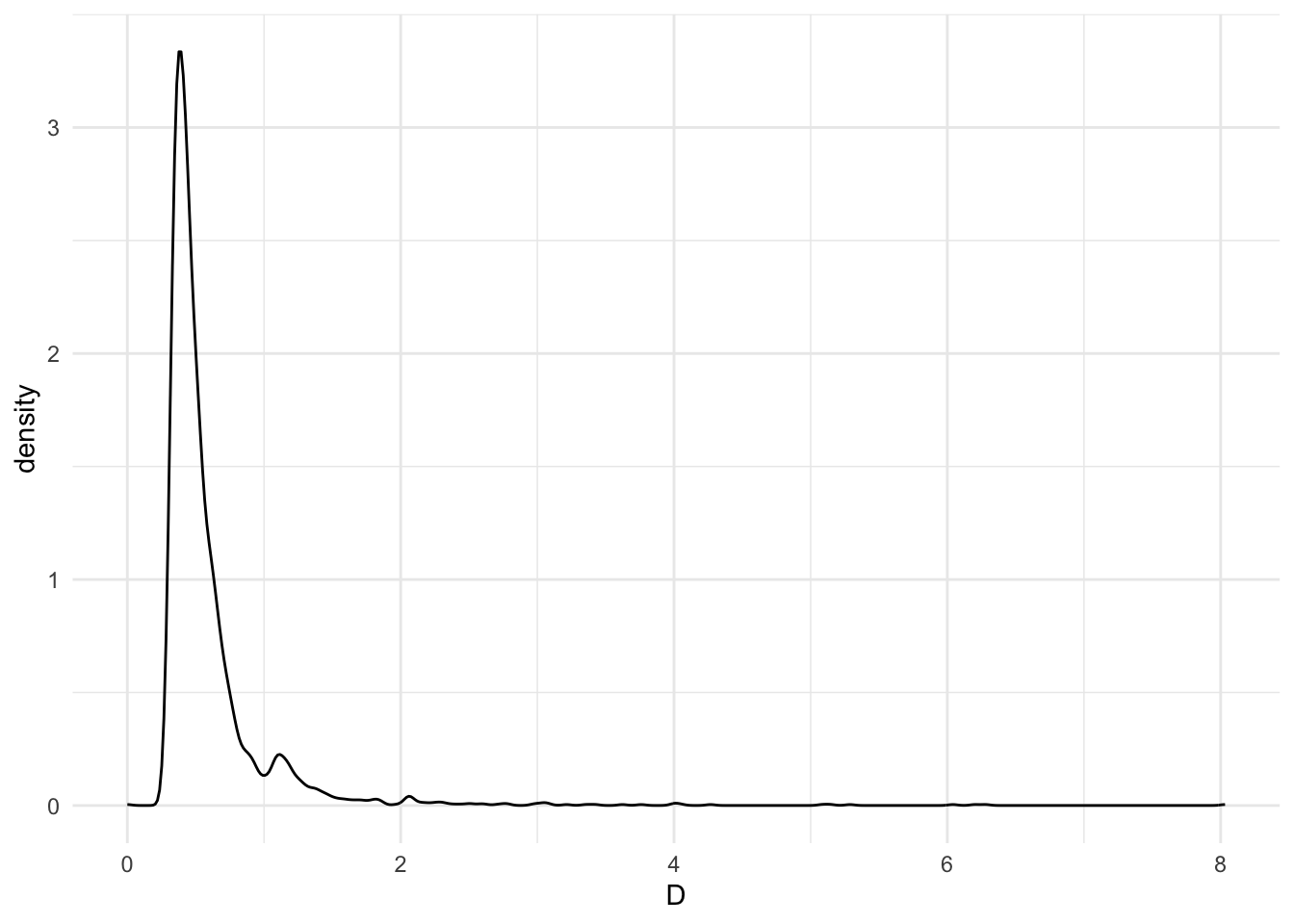
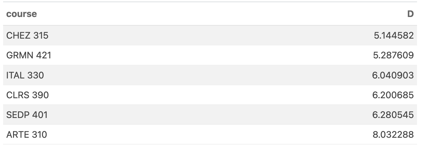
The five closest courses to ENVS 101, linguistically, are:

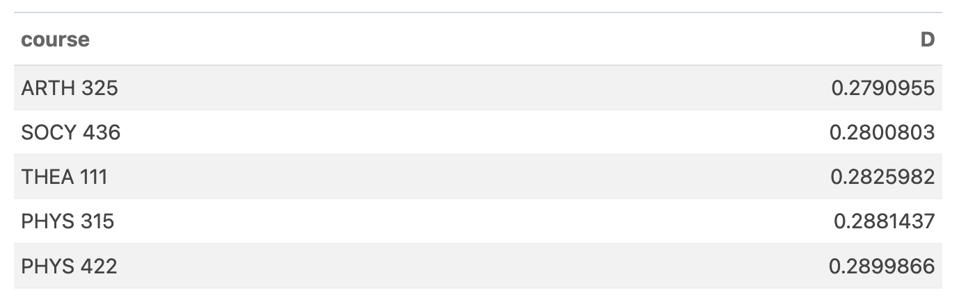
This is odd; why is art history the closest thing to an introduction to environmental studies?

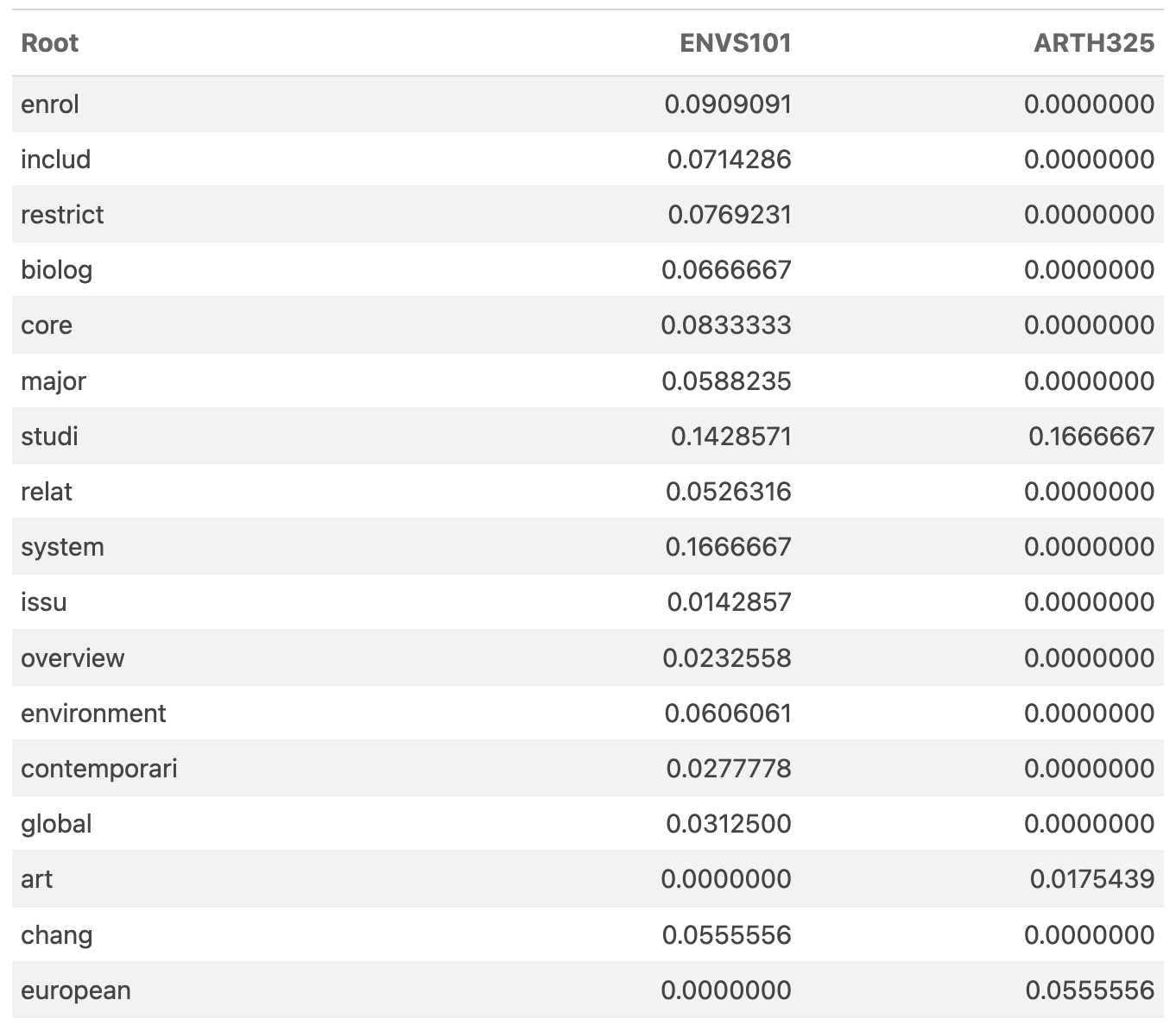
The distances from ENVS 101 (above) are dominated by course distances under 1.0. However, let's look closer at the actual mapping of linguistic components between ENVS 101 and ARTH 325. If we ignore the axes with no values (e.g., those that map onto linguistic stem components that are not in the course description) and look at only those that either course has non-zero data, we see that there are 17 non-zero points (in common). There is only 1 component studi that both courses share!

This is why pairwise similarity is not necessarily guaranteed to give you the best relationship—and where conditional covariance becomes much more informative because it is not defined on the magnitude of differences but rather the covariance of the two courses given their simultaneous relationship with all other classes. More on this later.

The courses that are most distant from ENVS 101 are:

We will skip the ENVS 101/ARTE 310 axis loadings for brevity.

Scale

Programs may require the same class but an alternate amount of credits. Since I normalize each course axis (e.g., the distance from the origin to the point for each course is scaled to = 1.0) and then weigh the contribution of each course by the number of classes needed, this impacts the hypervolume of the program in this high-dimensional space. You can think of the hypervolume if we enclosed all the points in solid; the volume of the included space is a measure of the linguistic diversity of the program (foreshadowing? perhaps).

However, two programs that require the same courses but with different credit requirements will have different hypervolumes (and hence shapes) in this linguistic space.

Population Graph Construction

The algorithm is provided in the PopGraph package (GitHub) and is general enough to use outside of a genetic context. It takes a vector of groupings (designating the node identity in the layout) and a multivariate data matrix.

load("data/stemmed_classes.rda")
numCols <- ncol( stemmed_classes)
degrees <- df$Program
stemmed_classes[0,] -> data
data$AcademicProgram <- character(0)

for( i in 1:length( degrees ) ) {
  program <- degrees[i]
  core <- programs[[program]]
  classes <- stemmed_classes[ stemmed_classes$Course %in% core , ]
  for( j in 1:nrow(classes) ) { 
      code <- classes$Course[j]
      credits <- as.numeric( vcu_courses$credits[ vcu_courses$class == code ] )  
      if( !is.na( credits) ) { 
        for( k in 2:ncol(classes)) {
          classes[j,k] <- classes[j,k] * (credits + 1)
        }  
      }
      else { 
        cat(program,code,"\n")
      }   
  }
  classes$AcademicProgram <- degrees[i]
  data <- rbind( data, classes )
}

And then visualize it using ggplot as:

library( popgraph )
library( ggrepel )
groups <- data$AcademicProgram

data |>
  select( -AcademicProgram, -Course) |>
  as.matrix() -> M

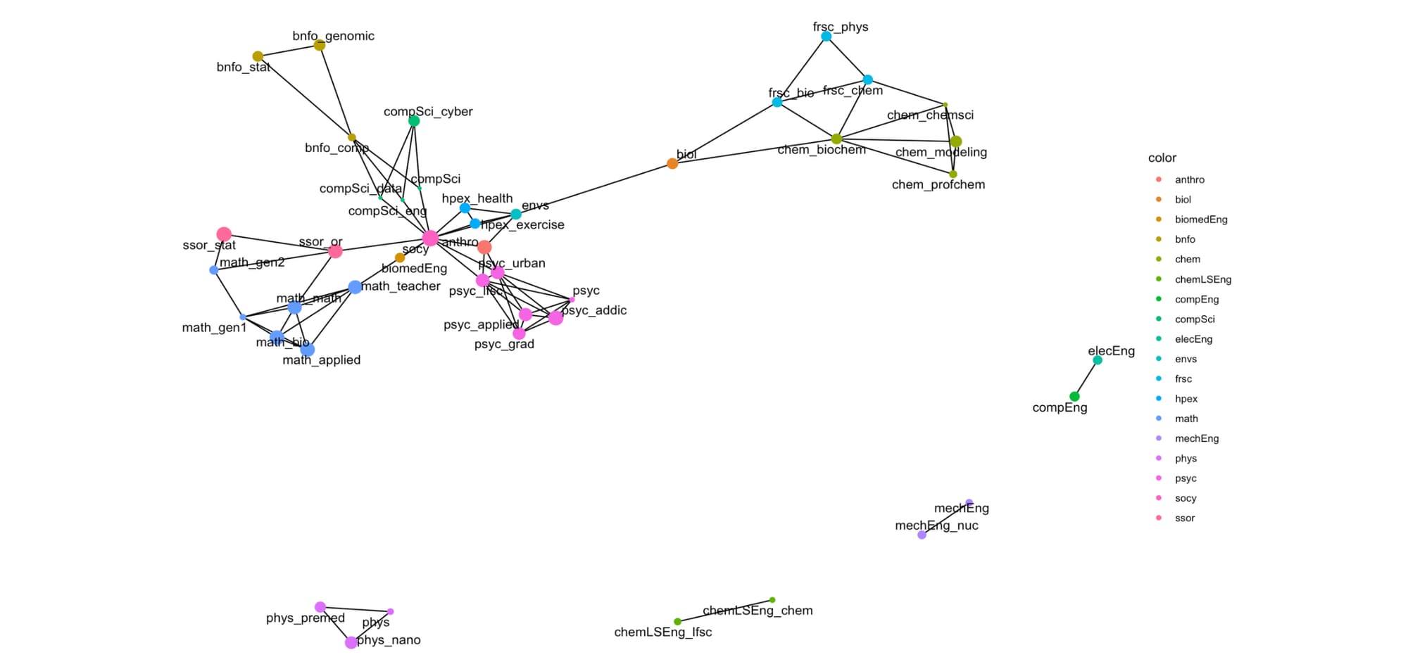
popgraph( M, groups = groups ) -> pg

coords <- igraph::layout_with_fr( pg )
V(pg)$x <- coords[,1]
V(pg)$y <- coords[,2]
V(pg)$Program <- stringr::str_split( V(pg)$name, pattern ="_", simplify = TRUE )[,1]

df.labels <- data.frame( Population=V(pg)$name, 
                         x = coords[,1], 
                         y = coords[,2])

pg <- decorate_graph(pg, df.labels)

ggplot() + 
  geom_edgeset( aes(x=x,y=y), graph = pg ) +
  geom_nodeset( aes(x=x,y=y, size=size, color=Program), graph = pg ) + 
  geom_text_repel( aes(x=x,y=y,label=Population), data = df.labels ) + 
  theme_void()

I colored the nodes by the program (so subprograms are all the same color), and the size of the major is proportional to the program's linguistic hypervolume of the node for a (e.g., a measure of diversity).

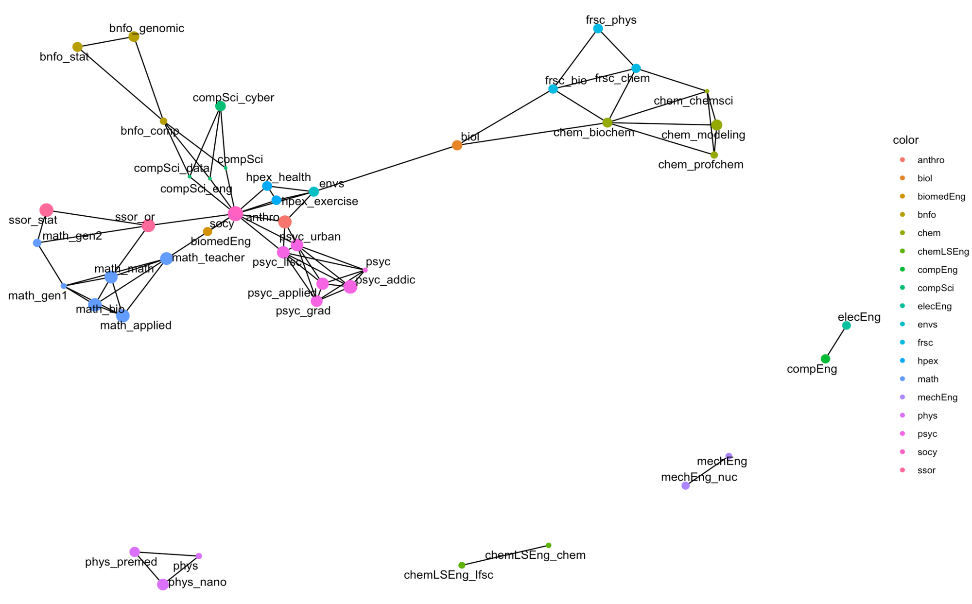
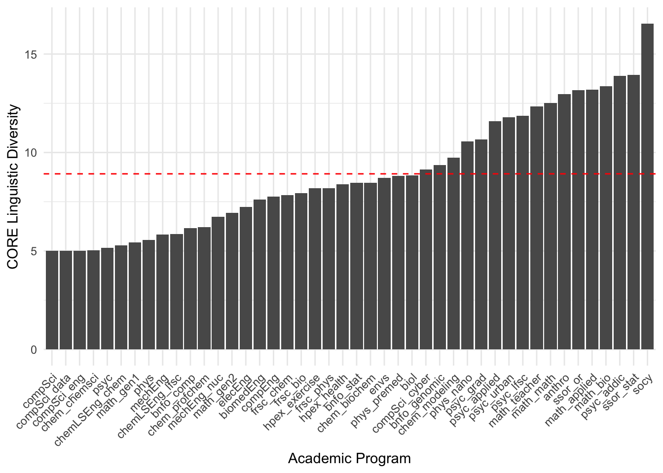
The diversity within programs (as defined by the node size above) varies across programs. Here is an ordered listing of them in increasing linguistic diversity. 

data.frame( Program = V(pg)$name,
            Diversity = V(pg)$size ) |>
  arrange( Diversity ) -> df 
df$Program <- factor( df$Program, ordered=TRUE, levels = df$Program )

df |> 
  ggplot( aes(Program,Diversity) ) + 
  geom_col() +
  scale_x_discrete(guide = guide_axis(angle = 45)) +
  geom_hline( yintercept = mean( V(pg)$size ), col="red", lty=2) + 
  xlab("Academic Program") + ylab("CORE Linguistic Diversity") +
  theme_minimal()

Conclusion

Exploring linguistic mapping within academic programs reveals a complex and nuanced landscape of educational structures, as depicted by the 44 STEM programs at VCU. By leveraging advanced techniques like word embeddings, we can gain deeper insights into the semantic relationships and contextual nuances of course offerings across various disciplines. Methods such as Word2Vec, as discussed earlier, provide a robust framework for understanding how words—and, by extension, courses—relate to one another within a high-dimensional space and will be added to this analysis in a subsequent posting. This approach allows us to comprehend academic programs' diversity and interconnectedness better, removing preceptor bias as it focuses on CORE components of the programs as standardized by SCHEV. There are some interesting findings in this topology, including:

1. Centrality: The topology's most central positions are those programs with the highest multidisciplinarity. This topology contains ENVS, HPEX, ANTRHO, and SOCY. Centrality is a critical component of independence graphs, which we will return to and discuss in subsequent posts. 
2. Independent Arms: Notice the general structure of the topology as a central core with the following arms:
   1. BIOL, FRSC, and CHEM occupy positions connected via a pendant to the remaining significant component of the topology. 
   2. Bioinformatics is situated outside of computer science. 
   3. Psychology and its sub-degrees are all co-located.
   4. Mathematics and Statistics similarly radiate from the core.
3. Isolated Subgraphs: The engineering and physics programs are disconnected. These programs (essentially) specify a set of requirements that are not shared with other programs—indeed, many of the Engineering programs here have very few options for electives, which centralize their entire CORE program in linguistic space—independent of the other programs.

The focus here is on the shape and placement of programs within the topology. The resulting topology of academic programs offers a compelling method for representing the diversity within and differences and interrelatedness between disciplines. In the coming blog posts, I will highlight how this approach enhances our understanding of academic programs and opens up new avenues for innovation in curriculum design.