Frequency-Dependent Linguistic Embedding of Course Descriptions
Mapping textual input into quantitative spaces facilitates statistical analyses supporting decision analytics. Here, university course descriptions are mapped onto numerical spaces and used to define the landscape of academic offerings.


As part of my book project, Intentional Curriculum Design: Data-Centric Approaches for STEM Curricula, I am analyzing the current landscape of university curricula based on CORE classes—those offerings in each degree program that all students must take. This post demonstrates the methods required to map the set of all course descriptions at Virginia Commonwealth University into quantitative spaces that can be used for statistical analysis.
Briefly, the goals of this post are to:
- Describe how to pre-process the text using standard linguistical methods.
- Extract features of all courses based upon linguistic stemming for each course offering and collate the data based on global frequency dependence.
- Examine the properties and characteristics of this quantitative space using ordination and hierarchical clustering.
The results of this work will be combined with mappings based on semantic meaning (in the next post), which forms the sample space on which the CORE curriculum of STEM programs can be extracted and their covariance can be quantified.
Embedding Language Components
To use course descriptions as a measure of academic program structure, one must first define a mapping of the original text for each course description onto a numerical space to examine the relative positions of the set of CORE classes from all degree programs. For the initial embedding,
- Text Preprocessing: We take raw text and pre-process it for analysis.
- Tokenization: Breaking down text into individual words or phrases.
- Stopword Removal: Eliminating common words that don't add much meaning, like "and" or "the."
- They are stemming/Lemmatization: Reducing words to their base or root form.
- Feature Extraction: Take the core elements of each item and map them into a high-dimensional numerical space. Both approaches can provide a high-dimensional coordinate vector for each course.
- Frequency-Dependent Analyses: Measures the importance of a word in a document relative to a collection of documents.
- Word Embeddings: Techniques like
Word2Vec,GloVe, andFastTextcapture semantic meanings of words in vector form. Of these three approaches,Word2Vecis best suited for our purposes. TheGloVeapproach focuses more on the global context. WhereasFastTextis more robust when handling out-of-vocabulary words, which we do not have.
Once the raw text is transferred into a common quantitative space, we can proceed with classification and examining covariance in topic coverage (to be handled in the next post).
Text Preprocessing
To pre-process text, we must remove all the text, break it into words by class description, remove non-informative words (such as 'and', 'but', etc.), and stem them.
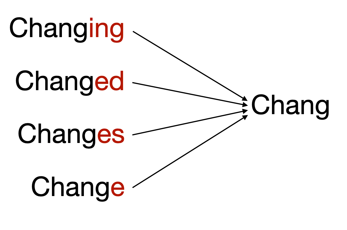
Stemming is the process of reducing inflected form of a word to one so-called “stem,” or root form, this is similar to “lemmatization”, though the base word is not reconstructed, just the core component.
An example is below, showing several words derived from the same stem.
I'll walk you through it so you can get the idea, then create a function to run through all the data.
rm( list=ls() )
load("data/vcu_courses.rda")
names( vcu_courses )
[1] "Index"    "class"    "title"    "hours"    "contact"  "credits"  "prereqs"
[8] "bulletin"
I'll grab the first one.
course <- vcu_courses$bulletin[1]
course
[1] "Enrollment is restricted to students in the biomedical engineering department and requires permission of course coordinator. This course involves the introduction of clinical procedures and biomedical devices and technology to biomedical engineering freshmen. Students will tour medical facilities, clinics and hospitals and will participate in medical seminars, workshops and medical rounds. Students will rotate among various programs and facilities including orthopaedics, cardiology, neurology, surgery, otolaryngology, emergency medicine, pharmacy, dentistry, nursing, oncology, physical medicine, ophthalmology, pediatrics and internal medicine."
Several libraries are used for this. I'm going to include them all here.
library( tm )
library( ape )
library( knitr )
library( tidyverse )
library( SnowballC )
library( kableExtra )
Most of the text manipulation components use a standard input type derived from a data.frame called a Corpus. Each document has its ID (in this case, the class name) and the raw text.
df <-  data.frame( doc_id = vcu_courses$class[1:2],
                   text = vcu_courses$bulletin[1:2] )
summary( df )
    doc_id              text
 Length:2           Length:2
 Class :character   Class :character
 Mode  :character   Mode  :character
Next, we will apply transformations to these entities by mapping various text manipulation functions. Most of the content_transformer() functions are self-explanatory.
corpus <- Corpus( DataframeSource( df ) )
corpus <- tm_map( corpus, content_transformer( removePunctuation ) )
corpus <- tm_map( corpus, content_transformer( tolower ) )
corpus <- tm_map( corpus, content_transformer( removeNumbers ) )
corpus <- tm_map( corpus, content_transformer( stripWhitespace) )
corpus <- tm_map( corpus, content_transformer(
  function(x) { removeWords( x, stopwords(kind="en") ) }
) )
corpus <- tm_map( corpus, content_transformer(
  function(x) { removeWords( x, stopwords( kind="SMART" ) ) }
) )
What this does is take the description for each course from;
vcu_courses$bulletin[1]
[1] "Enrollment is restricted to students in the biomedical engineering department and requires permission of course coordinator. This course involves the introduction of clinical procedures and biomedical devices and technology to biomedical engineering freshmen. Students will tour medical facilities, clinics and hospitals and will participate in medical seminars, workshops and medical rounds. Students will rotate among various programs and facilities including orthopaedics, cardiology, neurology, surgery, otolaryngology, emergency medicine, pharmacy, dentistry, nursing, oncology, physical medicine, ophthalmology, pediatrics and internal medicine."
And converts it to these words
corpus[[1]]$content
[1] "enrollment restricted students biomedical engineering department requires permission coordinator involves introduction clinical procedures biomedical devices technology biomedical engineering freshmen students tour medical facilities clinics hospitals participate medical seminars workshops medical rounds students rotate programs facilities including orthopaedics cardiology neurology surgery otolaryngology emergency medicine pharmacy dentistry nursing oncology physical medicine ophthalmology pediatrics internal medicine"
Now, we can stem these words
stemmed <- stemDocument( corpus[[1]] )
stemmed$content
[1] "enrol restrict student biomed engin depart requir permiss coordin involv introduct clinic procedur biomed devic technolog biomed engin freshmen student tour medic facil clinic hospit particip medic seminar workshop medic round student rotat program facil includ orthopaed cardiolog neurolog surgeri otolaryngolog emerg medicin pharmaci dentistri nurs oncolog physic medicin ophthalmolog pediatr intern medicin"
Then, we can save them back to the corpus.
for( i in 1:length(corpus)) {
  x <- corpus[[i]]
  y <- stemDocument( x )
  corpus[[i]] <- y
}
Next, we can turn this corpus into a term matrix, which records the number of occurrences of each stem in each document.
tdm <- TermDocumentMatrix( corpus )
m <- as.matrix( tdm )
head( m )
           Docs
Terms       EGRB 101 EGRB 102
  biomed           3        3
  cardiolog        1        0
  clinic           2        0
  coordin          1        0
  dentistri        1        0
  depart           1        0
These are the frequency spectra for stemmed words by course and are one numerical mapping of descriptions onto a numerical space for analysis. Here is all the code to do this (and a few other cleaning-up steps to make the data prettier).
#' This function assumes that df has two columns:
#'   - doc_id: A unique identification for each coruse (e.g., the code)
#'   - text: The raw bulletin text
filter_and_stem <- function( df, standardize=TRUE, verbose=FALSE ) {

  corpus <- Corpus( DataframeSource( df ) )
  corpus <- tm_map( corpus, content_transformer(removePunctuation))
  corpus <- tm_map( corpus, content_transformer(tolower))
  corpus <- tm_map( corpus, content_transformer(removeNumbers ))
  corpus <- tm_map( corpus, content_transformer(stripWhitespace))
  corpus <- tm_map( corpus, content_transformer(
    function(x) { removeWords(x, stopwords(kind="en")) } ))
  corpus <- tm_map( corpus, content_transformer(
    function(x) { removeWords(x, stopwords(kind="SMART")) } ))


  # Stem each document
  for( i in 1:length(corpus) ){
    x <- corpus[[i]]
    y <- stemDocument( x )
    corpus[[i]] <- y
  }

  # Turn it into a matrix and keep terms
  tdm <- TermDocumentMatrix( corpus )
  m <- as.matrix( tdm )

  # Keep only terms that are in at least 1% of the courses.
  cat("Stemmed Terms:",nrow(m),"\n")
  n <- m
  n[ n > 0 ] <- 1
  r <- rowSums( n )
  m <- m[ r > round(nrow(df) * 0.01) ,]

  # Normalize the stem count vectors to unit length
  r <- matrix( colSums( m ), nrow=nrow(m), ncol=ncol(m))
  m <- m / r

  cat("Retained Terms:",nrow(m),"\n")
  data <- data.frame( t(m) )

  data$Course <- rownames(data)
  data |>
    select( Course, dplyr::everything() ) -> data
  rownames(data) <- 1:nrow(data)
  return( data )
}
OK, now let's run all K = 2827 courses through this translation.
vcu_courses |>
  dplyr::select( doc_id = class,
          text = bulletin) -> df

filter_and_stem( df ) -> stemmed_classes
Stemmed Terms: 5733
Retained Terms: 565
Reprojecting Into Lower Dimensional Spaces
OK, so let's start by looking at the data to see what we have.
stemmed_classes |>
  str()
'data.frame':	2827 obs. of  566 variables:
 $ Course           : chr  "EGRB.101" "EGRB.102" "EGRB.104" "EGRB.105" ...
 $ clinic           : num  0.0645 0 0 0 0 ...
 $ coordin          : num  0.037 0 0 0 0 ...
 $ depart           : num  0.0175 0 0 0 0 ...
 $ emerg            : num  0.0526 0 0 0 0 ...
 $ engin            : num  0.087 0.8571 0.6667 0.6 0.0187 ...
 $ enrol            : num  0.05 0 0.167 0 0 ...
 $ includ           : num  0.0263 0 0.1429 0.0769 0 ...
 $ intern           : num  0.0323 0 0 0 0 ...
 $ introduct        : num  0.0476 0.0833 0 0 0 ...
 $ involv           : num  0.0312 0 0 0 0 ...
 $ medic            : num  0.15 0 0 0.05 0 0 0 0 0 0 ...
 $ medicin          : num  0.167 0.143 0 0 0 ...
 $ particip         : num  0.0312 0 0 0 0 ...
 $ permiss          : num  0.111 0 0 0 0 ...
 $ physic           : num  0.0172 0 0 0 0 ...
 $ procedur         : num  0.0182 0 0 0 0 ...
 $ program          : num  0.0417 0 0 0 0 ...
 $ requir           : num  0.0435 0 0.1 0 0 ...
 $ restrict         : num  0.05 0 0.0476 0 0 ...
 $ seminar          : num  0.0357 0 0 0 0 ...
  [list output truncated]
One of the first things to do is look at the data. However, as shown above, we have many of them (2827 classes and 565 stemmed terms). So, taking a direct look at it may be problematic. However, a common way to visualize high-dimensional data is to project it into a lower-dimensional representation. Here, I'll use a principal component approach to reproject the data under the constraints that the new axes I'll be looking at will be linear combinations of the previous ones selected to maximize the variation along the newly defined axes.
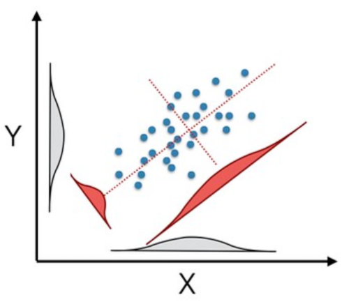
It is often helpful because the new axes describe decreasing variation in the data set while not impacting the relationship between the individual data points. This reprojection produces as many new axes as you had initially been, just sorted in relative importance defined by the amount of variation explained. As such, it can be a helpful way to take high-dimensional data and visualize it in a lower-dimensional space.
For this, I'll scale the data.
stemmed_classes |>
  select( -Course ) |>
  scale() -> pcadata
Then, we can run the analysis and take a look at the proportion of variation explained by each of the new composite axes:
library( factoextra )
fit.pca <- princomp( pcadata, cor = TRUE )
Let's start by taking a look at the importance of each axis (where importance is the fraction of the total variation in the data set explained by this axis):
fviz_eig( fit.pca, addlabels = TRUE, ncp = 10 )
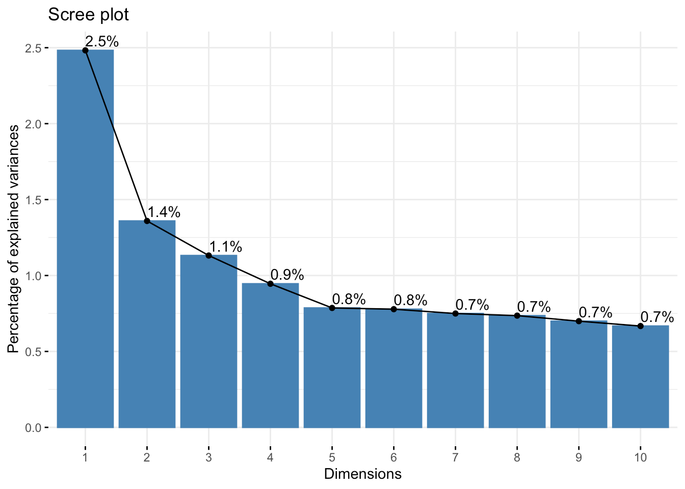
After the first four, it kind of levels out and slowly decreases.
Individual Axis Importance
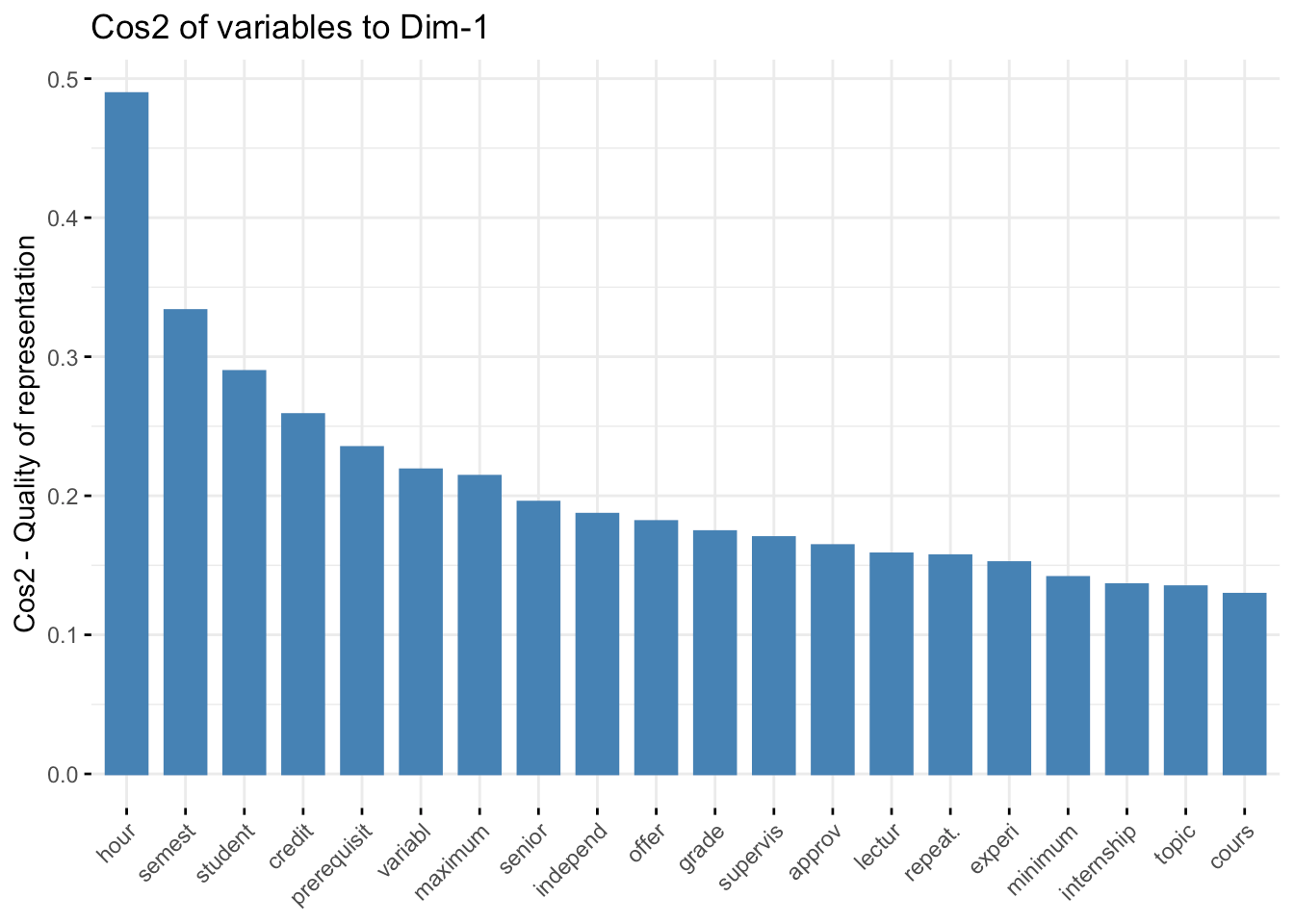
Next, let's look at the first component axes and what features of the original data set they use to define this new coordinate space. The first one loads (e.g., uses components from the original data) from the following original data axes (I've limited it to 20 for brevity):
fviz_cos2( fit.pca, choice="var", axes = 1,top = 20 )
The second axis loads onto:
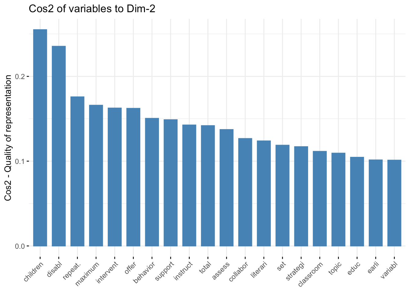
fviz_cos2( fit.pca, choice="var", axes = 2,top = 20 )
The third one uses:
fviz_cos2( fit.pca, choice="var", axes = 3,top = 20 )
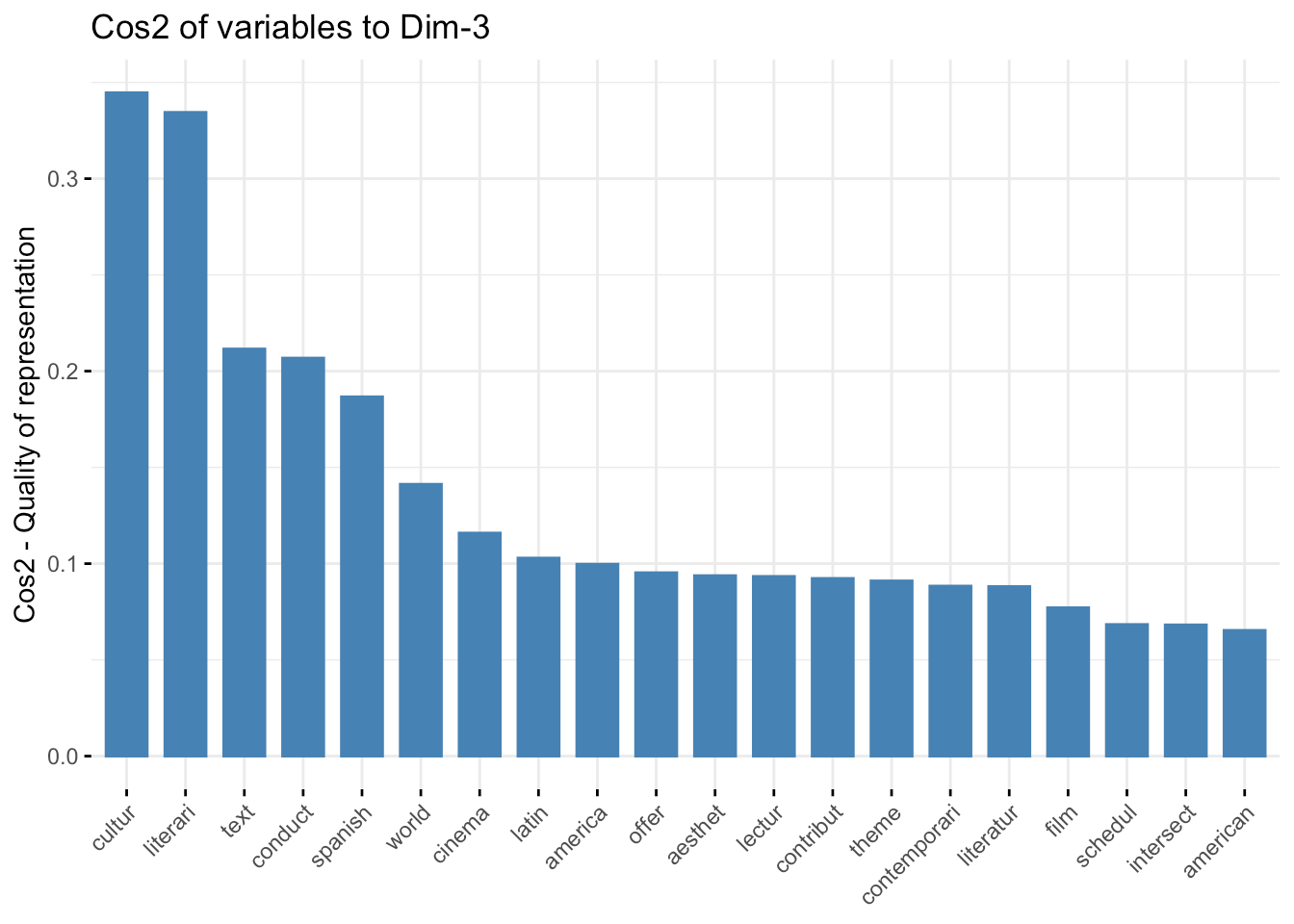
Qualitatively, the first axis seems to be primarily a housekeeping feature of common course descriptions, whereas the second and third axes appear to focus more on domain-specific components. It will be interesting when we reach into this background data set and localize the courses and linguistic spaces that define individual STEM programs at VCU (this will be in the next installment).
Individual Course Projections
Let's examine the individual courses as projected onto these new component axes. Remember, we have 2827 in the data set, so there will be too many points to get an in-depth overview. I'm adjusting this by setting alpha transparency so you can understand where things are piled up on each other.
Here are the first three axes.
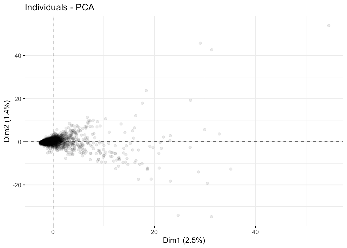
fviz_pca_ind( fit.pca, axes =c(1,2),geom.ind = "point", alpha=0.1)
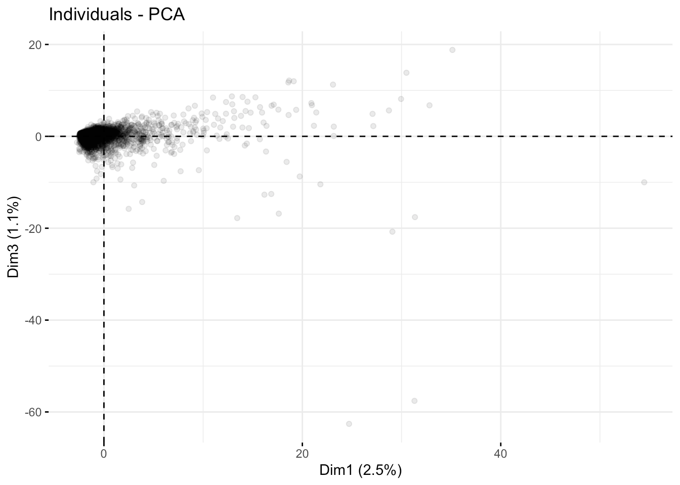
The first and third axes:
fviz_pca_ind( fit.pca, axes =c(1,3),geom.ind = "point", alpha=0.1)
And the second and third axes:
fviz_pca_ind( fit.pca, axes =c(2,3),geom.ind = "point", alpha=0.1)
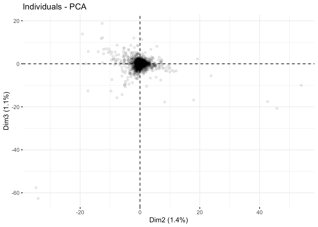
Overall, the course descriptions appear to have some outliers but no blatant compartmentalization, as depicted in the first few coordinate axes.
Hierarchical Clustering Analysis
Another way of looking at this is to take an unsupervised clustering approach and look at the hierarchy of similarities among the course descriptions. In general, an approach like this proceeds as follows:
- Identify the two most similar courses based on the linguistic projections of their descriptions.
- Create a node that combines these two and then throw it back into the pile (with N-1 entries since we combined them into a single entity).
- Identify the two most similar components and combine them, making N-2 entities.
- Continue until we have all the courses connected.
This is a greedy algorithm and a quick and dirty first approximation of how course semantics are clustered together. Still, it can reveal deep bifurcations in the data set that may not be obvious from examination of the first few principal component axes.
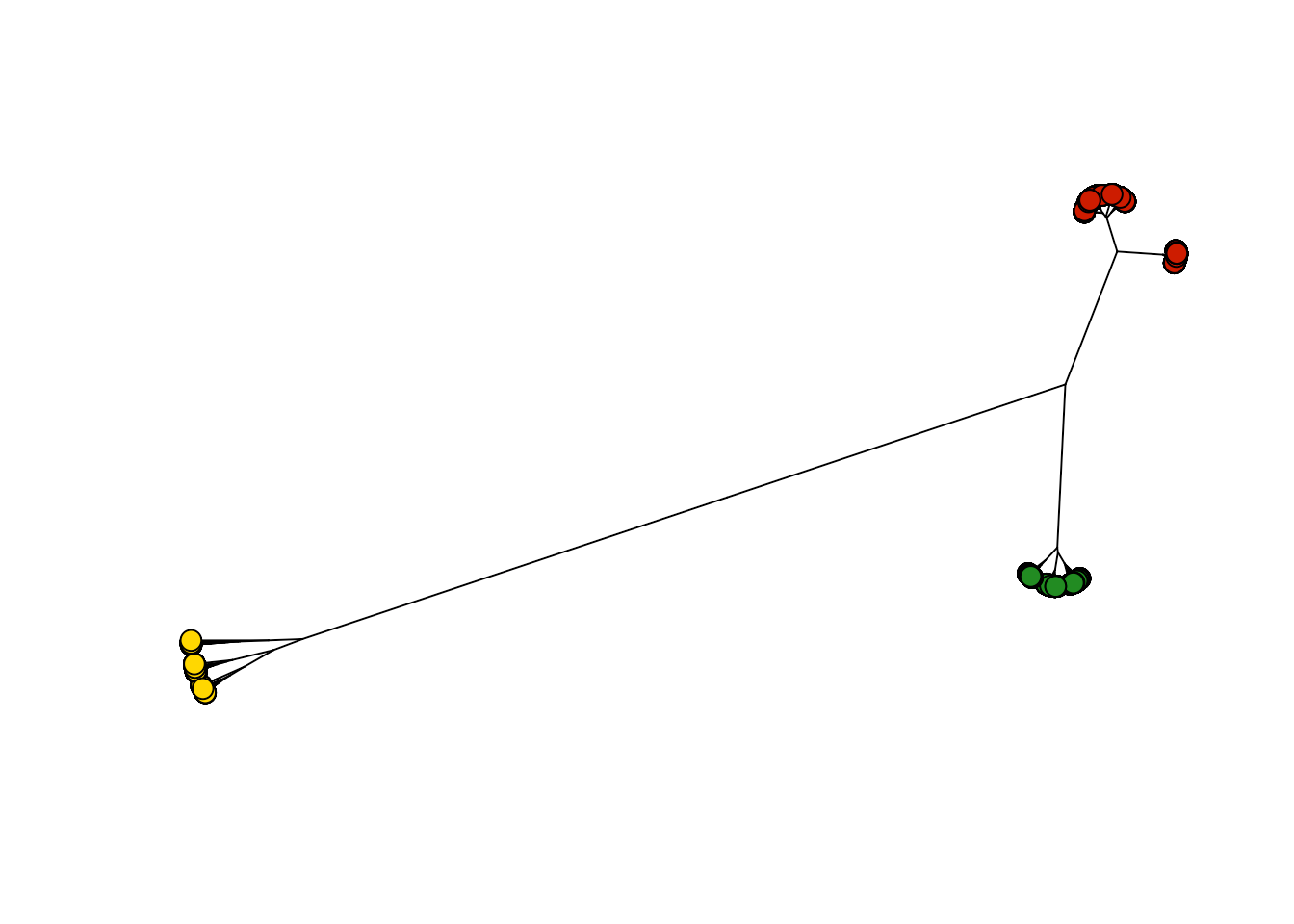
To begin with, we need to define a distance metric. I'm going to use a generic one based on Euclidean distances. To visualize this, I will make an unrooted tree and color the nodes by clusters. At first pass, it appears that there are three main groups of course descriptions, which I've colored in red, gold, and green.
D <- dist( stemmed_classes |> select( -Course ),
           method="euclidean")
hc <- hclust(D, method="ward.D" )
labelColors <- c("red3", "gold", "forestgreen")
groups <- cutree(hc, 3)
hcp <- as.phylo(hc)
plot( hcp, type="unrooted",  show.tip.label=FALSE, cex=0.5  )
tiplabels(pch=21, bg=labelColors[groups], cex=1.5)
Let's examine the courses in the groups. I'm going to remove the course numbers and just represent them by program designations (e.g., the class ENVS 101 will be represented by ENVS alone, independent of the course number). This is a gross simplification, as most curricula combine courses from several programs, but this at least will specify some compartmentalization.
course <- str_remove( stemmed_classes$Course, "[0-9]+")
course <- str_remove( course, "\\.")
course <- str_remove( course, "\\.")
course <- str_remove( course, "[0-9]+")
Some course listings appear divergent from the 4-letter + 3-number classification, so some cleaning was needed.
From this, I can construct a Venn diagram of the programs in each cluster.
df.courses <- data.frame( groups, course )
grp1 <- sort(unique(df.courses$course[ df.courses$groups == 1]))
grp2 <- sort(unique(df.courses$course[ df.courses$groups == 2]))
grp3 <- sort(unique(df.courses$course[ df.courses$groups == 3]))
VennDiagram::venn.diagram( x = list( grp1, grp2, grp3 ),
              category.names = c("Group 1", "Group 2", "Group 3"),
              filename = 'media/venn.png',
              output = TRUE ,
              imagetype="png" ,
              height = 480 ,
              width = 480 ,
              resolution = 300,
              compression = "lzw",
              lwd = 1,
              col= labelColors,
              fill = c( scales::alpha( labelColors[1], 0.3),
                        scales::alpha( labelColors[2], 0.3),
                        scales::alpha( labelColors[3], 0.3) ),
              cex = 0.5,
              fontfamily = "sans",
              cat.cex = 0.3,
              cat.default.pos = "outer",
              cat.pos = c(-27, 27, 135),
              cat.dist = c(0.055, 0.055, 0.085),
              cat.fontfamily = "sans",
              cat.col = labelColors,
              rotation = 1 ) -> tmp
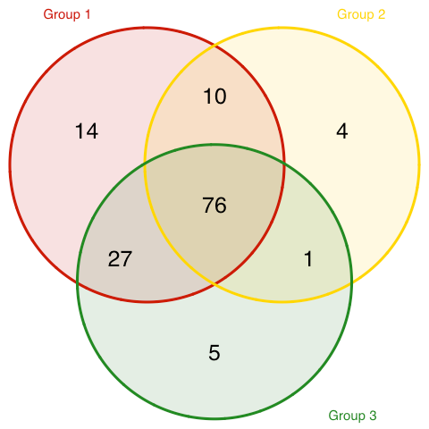
There is some overlap in program courses, but there are three sets of programs uniquely assigned to each of these three main clusters. Here are those programs.
progs1 <- setdiff( grp1, union(grp2, grp3) )
progs2 <- setdiff( grp2, union(grp1, grp3) )
progs3 <- setdiff( grp3, union(grp2, grp1) )

data.frame( Group = c("1", "2", "3"),
            Programs = c( paste( progs1, collapse=", "),
                          paste( progs2, collapse=", "),
                          paste( progs3, collapse=", ") ) ) |>
  kable() |>
  kable_paper(c("hover","striped"), full_width=F)
| Group | Programs |
|---|---|
| 1 | ANAT, ANTZ, ENVZ, EUCU, GRTY, HCMG, LASK, MEDC, MICR, NEXT, PATC, PHAR, PHTX, RHAB |
| 2 | CSIJ, MILS, PERI, PHIZ |
| 3 | FRSZ, GENP, HUS, LFSC, SSOR |
Looking at these program designations, I can see some points to classes that are not taught that often. One of the main assumptions in data treatment thus far is that the list of all 2827 courses are taught currently (or in the relatively recent past). As someone who has run one of these academic programs for the last decade, I can attest that a non-trivial fraction of the classes in the original list are not commonly offered.
Summary
As demonstrated above, it is reasonably easy to take a set of text components and map them onto a quantitative space that can be used for subsequent analyses. The goal here was to define the background data set, based upon all classes at Virginia Commonwealth University, that can be used to analyze the CORE class structure of all STEM curricula. In addition to these frequency-dependent approaches, the next installment will demonstrate how to extract semantic meaning from course descriptions, and together with the data presented here, we will be ready for the final set of analyses.